Here are the values of the density function stored as three dimensional, discrete grid, a big array. A possible source is for example the editor Acropora by Voxelogic. It can export it’s data as 3D DDS texture where each pixel can be interpreted as 32 bit float value. Naturally, the volume component supports it’s own optimized saving and loading of discrete grids, a later article covers this.
All in all, this article is quite math heavy, but every formula is simple on its own and can be literally translated into code, so don’t be scared.
Beside the density, it’s important to know what world dimensions the exported volume has. With all those data are the density and the gradient of a specific coordinate calculated. As preparation, the coordinate 


To give some options to the user to decide between loading time and quality, two methods to calculate the density and four for the gradient are given.
Calculating the density value can be done by interpolating via a “Nearest Neighbor” interpolation or a trilinear interpolation.
The nearest neighbor interpolates by simply choosing the grid coordinate which is closest to 

")
")
Although the nearest neighbor interpolation is very fast, a higher quality can be achieved by using the trilinear interpolation [Bou99]:
 = f_{000}(1 - x)(1 - y)(1 - z)+ f_{001}(1 - x)(1 - y)z \\ + f_{010}(1 - x)y(1 - z) + f_{011}(1 - x)yz \\ + f_{100}x(1 - y)(1 - z) + f_{101}x(1 - y)z \\ + f_{110}xy(1 - z) + f_{111}xyz")
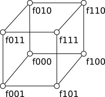
1: The vertices of a cube for trilinear interpolation
The range of x, y and z is from 0 to 1 with (0, 0, 0) being the vertex 

")

")
The gradient can be calculated either by using the nearest neighbor interpolation by evaluating ")
")
This is the Marching Cubes version:
 = \begin{pmatrix} G(x + 1, y, z) - G(x - 1, y, z) \\ G(x, y + 1, z) - G(x, y - 1, z) \\ G(x, y, z + 1) - G(x, y, z - 1) \end{pmatrix}")
The division by the cube length of the original version is left out here, because its 1 anyway in the grid.
A second possibility is the determination with a Sobel filter which adds a low pass filter and so is less prone to noise in the grid [Tö05, P. 176 – 178].
with
 = \begin{pmatrix} s_x(x, y, z) \\ s_y(x, y, z) \\ s_z(x, y, z) \end{pmatrix} / 4")
 = G(x + 1, y - 1, z) - G(x - 1, y - 1, z)) + \\ 2 \cdot (G(x + 1, y, z) - G(x - 1, y, z)) + \\ (G(x + 1, y + 1, z) - G(x - 1, y + 1, z)")
and
 = G(x, y + 1, z - 1) - G(x, y - 1, z - 1)) + \\ 2 \cdot (G(x, y + 1, z) - G(x, y - 1, z)) + \\ (G(x, y + 1, z + 1) - G(x, y - 1, z + 1)")
and
 - G(x - 1, y, z - 1)) + \\ 2 \cdot (G(x, y, z + 1) - G(x, y, z - 1)) + \\ (G(x + 1, y, z + 1) - G(x + 1, y, z - 1)")
Experience has shown, that the configuration with using trilinear interpolation for the density and nearest neighbor for the gradient without Sobel filter gives good results while keeping the loading time reasonable.