Volume Model | Volume GFX

The volume model is the base of all volume rendering. This is where the data comes from being transformed later into triangles.

Schaefer describes the volume model as density function f(x, y, z). The result of this function is the density or the distance to the surface of the model. The surface gets extracted by evaluating the function for a given density c: f(x, y, z) = c

With this kind of modelling, constructive solid geometry (CSG) becomes easy as only the function f(x, y, z) needs to be modified [SW04, S. 1].

c is also called the isovalue. The surface of the function at c is called isosurface [NY06, S. 1]. Typically, a isovalue of 0 is chosen. This way, negative densities are outside of the model and positive ones within.

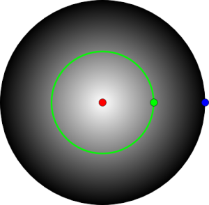
1: Visualization of a 2D circle volume

Picture 1 shows a two dimensional volume of a circle with the center $(x_c, y_c)$ and the radius r:

$f(x, y) = r - \sqrt{(x_c - x)^2 + (y_c - y)^2}$

White is the highest possible density r, marked with a red dot. At the green dot is the isovalue equal to 0, a mid gray in the image. All positions with an isovalue of 0 are marked in green and so a circle is created. The mapping of this isosurface with a mesh is called contouring [Hom10, S. 6]. Finally, the density function at the blue dot equals to -r.

The gradient at the given coordinate is also important. He will be used for the creation of an octree and for the lighting. The gradient is a vector with the components being the partial derivation of the density function. So the gradient is perpendicular to the isosurface. The length describes the amount of change of the function at the given position [Wei]. This is the gradient function of the two dimensional circle volume:

$\nabla f(x, y) = \begin{pmatrix} x \\ y \end{pmatrix} - \begin{pmatrix} x_c \\ y_c \end{pmatrix}$