Before there are any triangles generated in Dual Marching Cubes, there is still one big thing to be done: Deriving the Dualgrid from the Octree (generated in the previous article). Basically, it’s just a traversal over the Octree. This article is a bit long, but it is mostly a detailed description of the traversal, nothing really heavy.
But what is a Dualgrid? Duality in a mathematical sense means, that there is an object A and an object B, derived from A. If you create the dual object of B, it must be at least similar again to A [DLT].
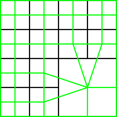
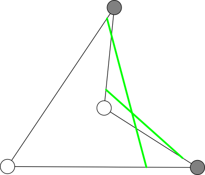
1: Two dimensional dualgrid
Figure 1 shows the two dimensional case with a Quadtree instead of an Octree, in black. The Dualgrid of this Quadtree is drawn in green [SW04, P. 3]
The Octree is traversed topdown and while doing so, some chosen features of the nodes become the Dualcells. All Dualcells together form the Dualgrid. Because of connecting nodes of different levels (the finer with the broader parts of the Octree), not only cubes are visually generated. Because some of the cell corners are on the exact same position, they degenerate to different forms. But there are always eight corners, so topological they are still cubes. In the two dimensional case above, the effect can be seen, too. There are not only rectangles, they degenerate to triangles for example. This is important later, when the triangles are generated [SW04, P. 5-6].
Too bad, Schaefer just describes in the paper the generation of the Dualgrid of a 2D quadtree and states, that the algorithm can be extended “naturally” to Octrees [SW04, P. 4]. But Holmlid gives a detailed explanation in his Master Thesis.
As a small reminder, here is the numbering of the Octree children again:
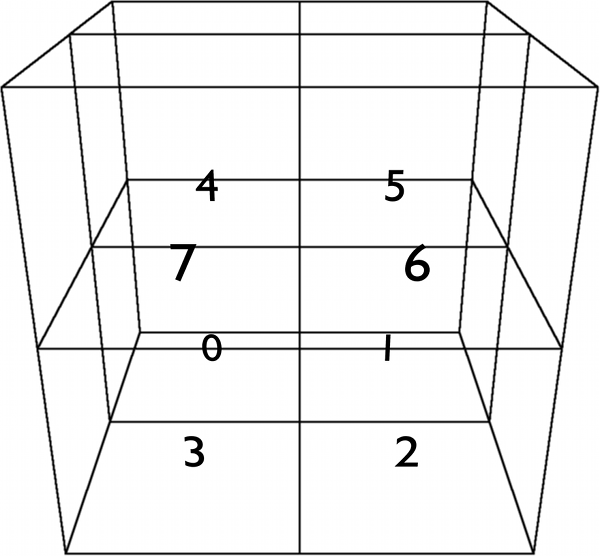
2: Numbering of the Octree children
The Recursive Functions
Four recursive functions traverse the Octree, nodeProc(n), faceProc(n0, n1), edgeProc(n0, n1, n2, n3) and vertProc(n0, n1, n2, n3, n4, n5, n6, n7). All parameters are Octree nodes. As Homlid did, some functions are defined like this:
edgeProc(n0, n1, n2, n3) in
- edgeProcX(n0, n1, n2, n3)
- edgeProcY(n0, n1, n2, n3)
- edgeProcZ(n0, n1, n2, n3)
faceProc(n0, n1) in
- faceProcXY(n0, n1)
- faceProcZY(n0, n1)
- faceProcXZ(n0, n1)
This way, the spatial relations are preserved without having a lot of case differentations.
When a node given to one of those functions doesn’t have children anymore, it is given itself as parameters instead. That’s why not only cubes but many different forms with vertices on top of each other appear as Dualcell and so Octree nodes of different tree levels are connected without dedicated knowledge of the neighbors [Hom10, P. 21-25].
nodeProc(n)
With this function, the recursion starts.
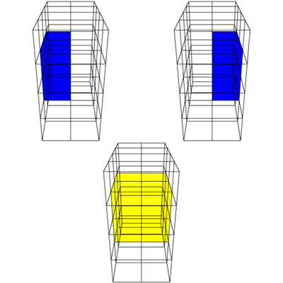
Figure 3 illustrates the calls to the functions nodeProc(n), faceProc(n0, n1), edgeProc(n0, n1, n2, n3) and vertProc(n0, n1, n2, n3, n4, n5, n6, n7).
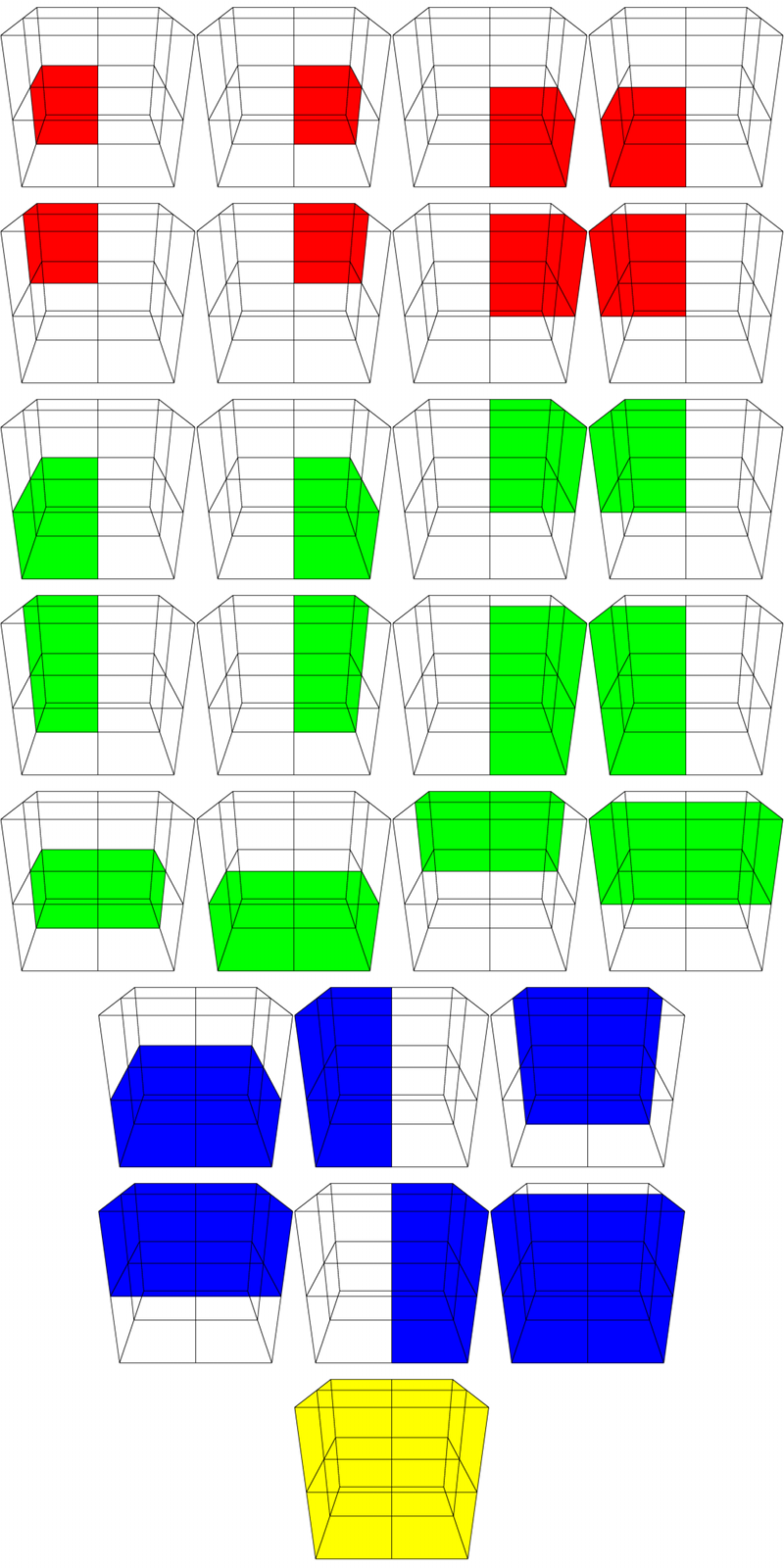
3: The calls of nodeProc(n) to the other functions
This is it’s pseudocode:
nodeProc(n) {
    if (n.isSubdivided()) {
        nodeProc(n.child(0));
        nodeProc(n.child(1));
        nodeProc(n.child(2));
        nodeProc(n.child(3));
        nodeProc(n.child(4));
        nodeProc(n.child(5));
        nodeProc(n.child(6));
        nodeProc(n.child(7));

        faceProcXY(n.child(0), n.child(3));
        faceProcXY(n.child(1), n.child(2));
        faceProcXY(n.child(4), n.child(7));
        faceProcXY(n.child(5), n.child(6));

        faceProcZY(n.child(0), n.child(1));
        faceProcZY(n.child(3), n.child(2));
        faceProcZY(n.child(4), n.child(5));
        faceProcZY(n.child(7), n.child(6));

        faceProcXZ(n.child(4), n.child(0));
        faceProcXZ(n.child(5), n.child(1));
        faceProcXZ(n.child(7), n.child(3));
        faceProcXZ(n.child(6), n.child(2));

        edgeProcX(n.child(0), n.child(3), n.child(7), n.child(4));
        edgeProcX(n.child(1), n.child(2), n.child(6), n.child(5));

        edgeProcY(n.child(0), n.child(1), n.child(2), n.child(3));
        edgeProcY(n.child(4), n.child(5), n.child(6), n.child(7));

        edgeProcZ(n.child(7), n.child(6), n.child(2), n.child(3));
        edgeProcZ(n.child(4), n.child(5), n.child(1), n.child(0));

        vertProc(n.child(0), n.child(1), n.child(2), n.child(3), n.child(4), n.child(5), n.child(6), n.child(7));
    }
}
faceProc(n0, n1)
This pseudocode just shows faceProcXZ(n0, n1), the other ones are analogue.
faceProcXY(n0, n1) {
    if (n0.isSubdivided() || n1.isSubdivided()) {
        c0 = n0.isSubdivided() ? n0.child(3) : n0;
        c1 = n0.isSubdivided() ? n0.child(2) : n0;
        c2 = n1.isSubdivided() ? n1.child(1) : n1;
        c3 = n1.isSubdivided() ? n1.child(0) : n1;
        c4 = n0.isSubdivided() ? n0.child(7) : n0;
        c5 = n0.isSubdivided() ? n0.child(6) : n0;
        c6 = n1.isSubdivided() ? n1.child(5) : n1;
        c7 = n1.isSubdivided() ? n1.child(4) : n1;

        faceProcXY(c0, c3);
        faceProcXY(c1, c2);
        faceProcXY(c4, c7);
        faceProcXY(c5, c6);

        edgeProcX(c0, c3, c7, c4);
        edgeProcX(c1, c2, c6, c5);

        edgeProcY(c0, c1, c2, c3);
        edgeProcY(c4, c5, c6, c7);

        vertProc(c0, c1, c2, c3, c4, c5, c6, c7);
    }
}
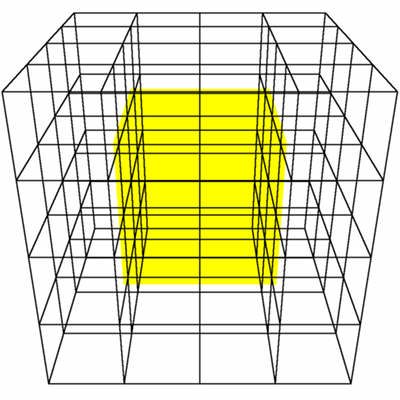
And the visualization:
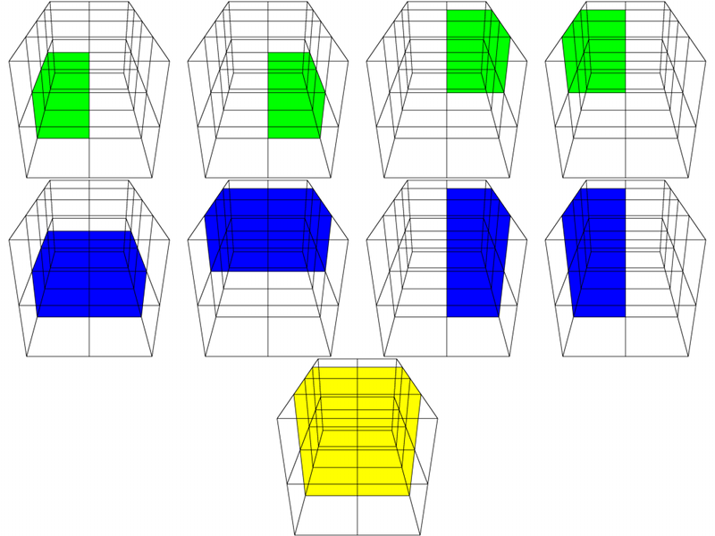
4: The calls of faceProc(n0, n1)
edgeProc(n0, n1, n2, n3)
The pseudocode is getting shorter. Again, only one version as the other ones are similar.
edgeProcX(n0, n1, n2, n3) {
    if (n0.isSubdivided() || n1.isSubdivided() || n2.isSubdivided() || n3.isSubdivided()) {
        c0 = n0.isSubdivided() ? n0.child(7) : n0;
        c1 = n0.isSubdivided() ? n0.child(6) : n0;
        c2 = n1.isSubdivided() ? n1.child(5) : n1;
        c3 = n1.isSubdivided() ? n1.child(4) : n1;
        c4 = n3.isSubdivided() ? n3.child(3) : n3;
        c5 = n3.isSubdivided() ? n3.child(2) : n3;
        c6 = n2.isSubdivided() ? n2.child(1) : n2;
        c7 = n2.isSubdivided() ? n2.child(0) : n2;

        edgeProcX(c0, c3, c7, c4);
        edgeProcX(c1, c2, c6, c5);

        vertProc(c0, c1, c2, c3, c4, c5, c6, c7);
    }
}
5: The calls of edgeProcX
vertProx(n0, n1, n2, n3, n4, n5, n6, n7)
When this function is reached and all given nodes are leafes, then a Dualcell is finally created.
vertProc(n0, n1, n2, n3, n4, n5, n6, n7) {
    if (n0.isSubdivided() || n1.isSubdivided() || n2.isSubdivided() || n3.isSubdivided() ||
        n4.isSubdivided() || n5.isSubdivided() || n6.isSubdivided() || n7.isSubdivided()) {
        c0 = n0.isSubdivided() ? n0.getChild(6) : n0;
        c1 = n1.isSubdivided() ? n1.getChild(7) : n1;
        c2 = n2.isSubdivided() ? n2.getChild(4) : n2;
        c3 = n3.isSubdivided() ? n3.getChild(5) : n3;
        c4 = n4.isSubdivided() ? n4.getChild(2) : n4;
        c5 = n5.isSubdivided() ? n5.getChild(3) : n5;
        c6 = n6.isSubdivided() ? n6.getChild(0) : n6;
        c7 = n7.isSubdivided() ? n7.getChild(1) : n7;
        vertProc(c0, c1, c2, c3, c4, c5, c6, c7);
    } else {
        if (!n0.isIsoSurfaceNear() && !n1.isIsoSurfaceNear() && !n2.isIsoSurfaceNear() && !n3.isIsoSurfaceNear() && !n4.isIsoSurfaceNear() &&
            !n5.isIsoSurfaceNear() && !n6.isIsoSurfaceNear() && !n7.isIsoSurfaceNear()) {
            return;
        }
        createDualCell(n0.center(), n1.center(), n2.center(), n3.center(), n4.center(), n5.center(), n6.center(), n7.center());
        createBorderCells(n0, n1, n2, n3, n4, n5, n6, n7);
    }
}
And one last recursive call is inside in the case one of the nodes is not a leafe.
6: The call of vertProc to itself in case the nodes are not all leafes
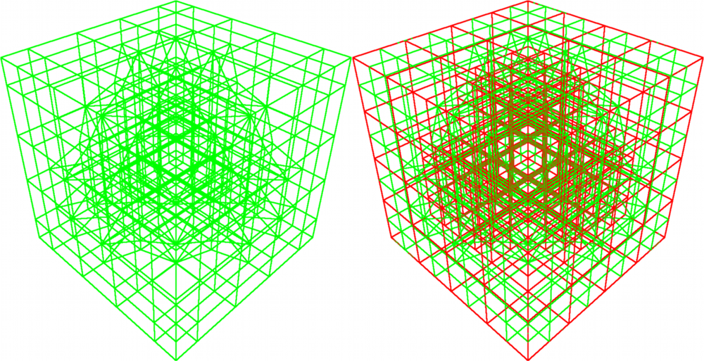
Without paying attention to the line with the condition that all nodes are near to the isosurface and the call to createBorderCells(n0, n1, n2, n3, n4, n5, n6, n7), the Octree of the quarter sphere becomes this Dualgrid:
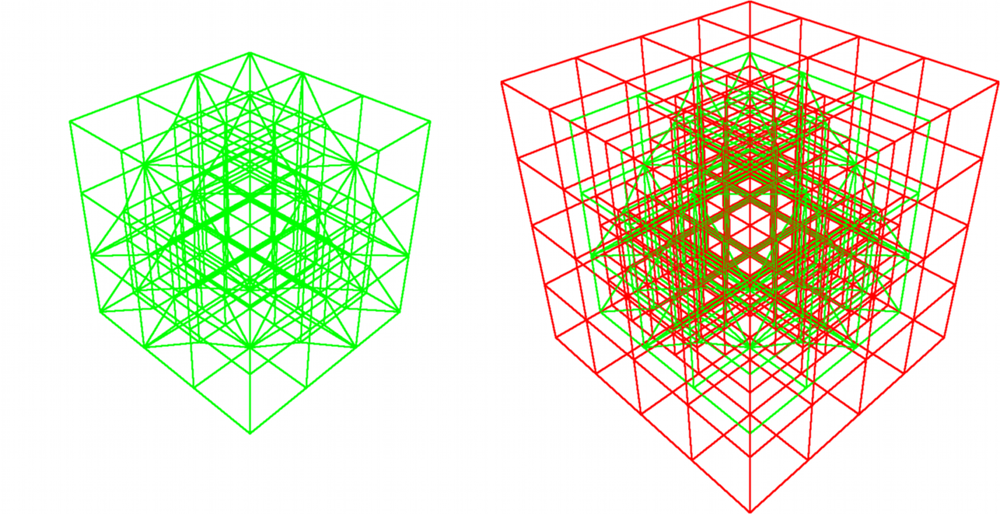
7: The Dualgrid of the quarter sphere so far
But we need only Dualcells if all children are somewhat near to the isosurface and so they have a chance to create some triangles later. This is how it looks like if this condition is taken in:
8: An adaptive Dualgrid
Notice that the center of the nodes are taken as vertices for the Dualcell. In the original Dual Marching Cubes, Schaefer calls this a feature of the cell and calculates an interesting point using again a QEF. This is how sharp edges are preserved in the algorithm [SW04, P. 3]. But this is really slow. On Schaefers 3 GHz Pentium, it took up to several minutes to isolate the features of a dragon model [SW04, P.6]. In addition, Manson and Schaefer later discovered, that overlapping triangles can be created if the Dualcell gets concave, see figure 6 [MS10, P. 2].
9: 2D concave Dualcell producing overlapping triangles
This is again a 2D Dualcell, but due to the QEF feature isolation, it gets concave. The dark corners are inside the volume, the bright ones outside. Green are the edges generated by Marching Squares (as it is 2D). They overlapp.
But Schaefer proposes just using the centers of the Octree nodes as an alternative [SW04, P. 6]. This way, no concave dualcells can appear. As the main application of this project is the visualisation of organic terrain and the loading time is also crucial, they are used here.
What’s still missing is the call to createBorderCells(n0, n1, n2, n3, n4, n5, n6, n7).
Creating border Dualcells
This is the last part of deriving the Dualgrid. As you might noticed, the Dualgrid in figure 7 doesn’t reach the borders of the Octree and so doesn’t cover the whole volume. Schaefer proposes to call edgeProc(n0, n1, n2, n3) and vertProc(n0, n1, n2, n3, n4, n5, n6, n7) again with degenerated Octree nodes. Degenerated means, that a 3x3x3 grid is taken where the outer cells collapse into planes and vertices (corner cells) [SW04, P. 4]. But this means, that the whole Octree has to be traversed again which would increase the loading time.
That’s why a different approach was chosen in this project. createBorderCells(n0, n1, n2, n3, n4, n5, n6, n7) checks the given nodes whether they are at the border and which of the following cases appear:
- The node is on an outer plane (6 possibilities)
- The node is on an outer edge (12 possibilities)
- The node is on an outer corner (8 possibilities)
That sums up to 26 border cases. The tests which possibility are given for a node reduce each other. An outer corner being left, top and back must be on the top plane and also on the back edge.
This pseudocode shows the handling of the back plane. The comments state the case.
// If the back ones of the eight nodes are at the back of the volume...
if (n0.isBorderBack() && n1.isBorderBack() && n4.isBorderBack() && n5.isBorderBack()) {
    // ...create the back Dualcell.
    createDualCell(n0->centerBack(), n1->centerBack(), n1->center(), n0->center(), n4->centerBack(), n5->centerBack(), n5->center(), n4->center()));
    // ...and the nodes 4 and 5 are at the top of the volume...
    if (n4.isBorderTop() && n5.isBorderTop()) {
        // ...create the edge Dualcell being at the top and back.
        createDualCell(n4.centerBack(), n5.centerBack(), n5.center(), n4.center(), n4.centerBackTop(), n5.centerBackTop(), n5.centerTop(), n4.centerTop());
        // ...and the node 4 is at the left of the volume...
        if (n4.isBorderLeft()) {
            // ...create the left back top corner Dualcell.
            createDualCell(n4.centerBackLeft(), n4.centerBack(), n4.center(), n4.centerLeft(), n4.getCorner4(), n4.centerBackTop(), n4.centerTop(), n4.centerLeftTop());
        }
        // ...and the node 4 is at the right of the volume...
        if (n5.isBorderRight()) {
            // ...create the right back top corner Dualcell.
            createDualCell(n5.centerBack(), n5.centerBackRight(), n5.centerRight(), n5.center(), n5.centerBackTop(), n5.getCorner5(), n5.centerRightTop(), n5.centerTop());
        }
    }
    // ...and the two nodes 0 and 1 are at the bottom volume border...
    if (n0.isBorderBottom() && n1.isBorderBottom()) {
        // ...create the bottom back edge Dualcell.
        createDualCell(n0.centerBackBottom(), n1.centerBackBottom(), n1.centerBottom(), n0.centerBottom(), n0.centerBack(), n1.centerBack(), n1.center(), n0.center());
        // ...and the node 0 is at the left of the volume...
        if (n0.isBorderLeft()) {
            // ...create the left back bottom corner Dualcell.
            createDualCell(n0.getFrom(), n0.centerBackBottom(), n0.centerBottom(), n0.centerLeftBottom(), n0.centerBackLeft(), n0.centerBack(), n0.center(), n0.centerLeft());
        }
        // ...and the node 1 is at the right of the volume...
        if (n1.isBorderRight()) {
            // ...create the right back bottom corner Dualcell.
            createDualCell(n1.centerBackBottom(), n1.getCorner1(), n1.centerRightBottom(), n1.centerBottom(), n1.centerBack(), n1.centerBackRight(), n1.centerRight(), n1.center());
        }
    }
}
A bit tedious, but after some time it works flawlessly. The creation of the border Dualcells for the front, left and right planes works similar. The treatment of the top and bottom planes is shorter because most of the edges and all corners are done already.
// If the top of the eight nodes are at the top of the volume...
if (n4.isBorderTop() && n5.isBorderTop() && n6.isBorderTop() && n7.isBorderTop()) {
    // ...create the top Dualcell.
    createDualCell(DualCell(n4.center(), n5.center(), n6.center(), n7.center(), n4.centerTop(), n5.centerTop(), n6.centerTop(), n7.centerTop()));
}
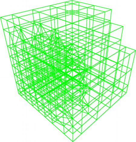
After writing if-statement after if-statement and paying a lot of attention to the cases, it’s done, the Dualgrid has its border cells!
10: The complete Dualgrid of the quarter sphere scene