Octree Generation | Volume GFX

The first part of Dual Marching Cubes is the generation of an Octree. All in all, this Octree is responsible for having less triangles in plane areas and more in curved. And with the parameters, it controls how much detail in general is created, how many triangles are used. But first, what is an Octree?

Octree Introduction

An Octree is a tree datastructure. It’s root is a world enclosing cube. The eight children recursivly splits it into eight octants, hence the name Octree. The splitting stops as soon as a certain heuristic is accomplished [DeL00, P. 439].

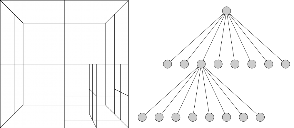
1: Example Octree

Look at figure 1, it shows an example Octree with it’s tree structure. Figure 2 illustrates the indices of the children being used here.

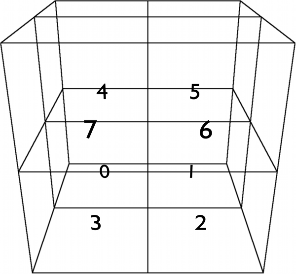
2: Numbering of the Octree children

Octree Generation

So we need to build an Octree which closely resembles the density function. As said, this is a recursive process based on a heuristic, being splitPolicy called here. It takes the current node and a tolerated geometric error as arguments and decides based on that information, whether to split the node into eight children or not. If splitted, the process begins again for every child.

void OctreeNode::split(const OctreeNodeSplitPolicy *splitPolicy, const Source *src, const Real geometricError)
{
    if (splitPolicy->doSplit(this, geometricError))
    {
        Vector3 newCenter, xWidth, yWidth, zWidth;
        OctreeNode::getChildrenDimensions(mFrom, mTo, newCenter, xWidth, yWidth, zWidth);
        mChildren = new OctreeNode*[OCTREE_CHILDREN_COUNT];
        mChildren[0] = createInstance(mFrom, newCenter);
        mChildren[0]->split(splitPolicy, src, geometricError);
        mChildren[1] = createInstance(mFrom + xWidth, newCenter + xWidth);
        mChildren[1]->split(splitPolicy, src, geometricError);
        mChildren[2] = createInstance(mFrom + xWidth + zWidth, newCenter + xWidth + zWidth);
        mChildren[2]->split(splitPolicy, src, geometricError);
        mChildren[3] = createInstance(mFrom + zWidth, newCenter + zWidth);
        mChildren[3]->split(splitPolicy, src, geometricError);
        mChildren[4] = createInstance(mFrom + yWidth, newCenter + yWidth);
        mChildren[4]->split(splitPolicy, src, geometricError);
        mChildren[5] = createInstance(mFrom + yWidth + xWidth, newCenter + yWidth + xWidth);
        mChildren[5]->split(splitPolicy, src, geometricError);
        mChildren[6] = createInstance(mFrom + yWidth + xWidth + zWidth, newCenter + yWidth + xWidth + zWidth);
        mChildren[6]->split(splitPolicy, src, geometricError);
        mChildren[7] = createInstance(mFrom + yWidth + zWidth, newCenter + yWidth + zWidth);
        mChildren[7]->split(splitPolicy, src, geometricError);
    }
}

The Heuristic

The used heuristic is based on an accepted geometric error as threshold. The (roughly approximated) error of the current node is calculated and it is split, when the calculated error is higher than the accepted geometric error.

Schaefer uses an heuristic based on Quadratic Error Functions (QEFs). He calculates planes on the points of an uniform grid spread over the node, builds with them a QEF and minimizes it as a quadratic function [SW04, P. 2 – 3]. This is an very expensive and complicated operation, so in this project uses a different approach.

It is developed by Zhang, Bajaj and Sohn. The geometric error of the current node is calculated with the difference of a trilinear interpolation and the real values on specific test points. The density values on the eight corners of the node are the base of the interpolation.

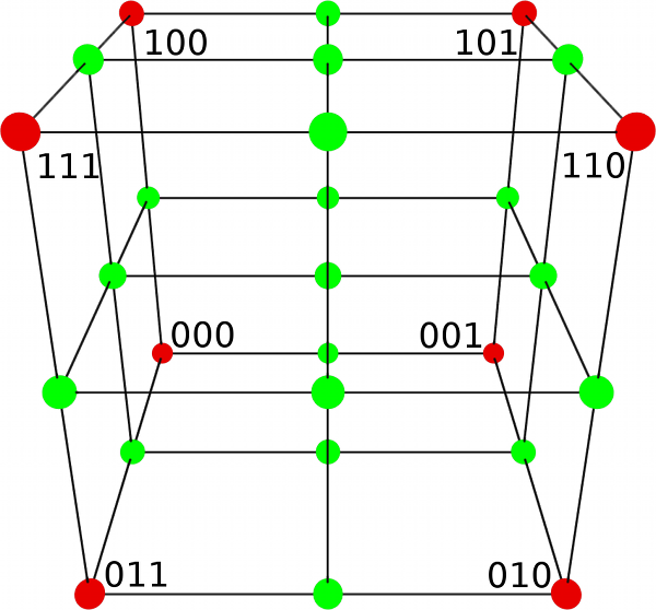
3: An Octree node with his red corners and all green corners of his children

In figure 3, they are shown as red dots. The corners of the potential children are marked in green. At those green points, the density values are taken from the density source and also trilinear interpolated. The same formula as in the discrete grid is used for the interpolation. Now, the difference between density value and interpolated value is calculated as follows. Here is the one dimensional case.

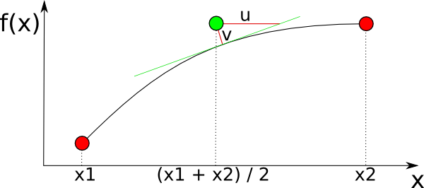
4: One dimensional error approximation between interpolation and function

The error is $v = \frac{u}{k}$ with k being the slope of the green tangent. In higher dimensions, k just becomes the length of the gradient vector. Pay attention to take a minimum of 1 as the slope or else, giant errors will sneak in. The thought behind this approximation of the distance of an interpolated value to the function is this: The higher the slope is, the steeper is the tangent, the higher must be the correction (the division).

Now the error can be calculated like this:

$Error = \sum \frac{|f^{i + 1} - f^i|}{|\nabla f^i|}$

With $f^{i + 1}$ as the interpolated value and $f^i$ the real density value, summed up over all green corners [ZBS05, S. 16-17].

A few optimizations can be done here: First, a minimum Octree node size is defined at the beginning. If the current node has reached it, the splitting is stopped without calculating the geometric error. And second, the splitting can be stopped if the center of the node is far enough away from the isosurface (like the Octree nodes diagonal length). Then it will never generate a triangle anyway. The last optimization is the constant checking of the current error against the tolerated one while summing it up. If the error reaches early the tolerated one, it can be stopped.

This is the result of a generated Octree for a quarter sphere being in an corner. Pay attention to the far bigger Octree cells being at the other corners where the splitting has stopped early.

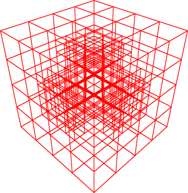
5: The Octree of a quarter sphere being in the corner